An interesting method of bandpass filter testing and tunung is described in Agilent AN 1287-8 (Simplified Filter Tuning Using Time Domain) and AN 1287-10 (Network Analysis Solutions Advanced Filter Tuning Using Time Domain Transforms) application notes. This method is based on S11 parameter convertion into the time domain.
By using a vector analyzer, a scan is performed at several hundred frequencies. The center frequency should be equal to the resonant frequency of the filter; the scan range should be 2..5 times (this is recommended by Agilent) larger than the bandwidth of the filter. The S11 paramers are converted into the time domain by using inverse Fourier transform, and the result is plotted at the graph (either in linear or logarithimic scale). The graph shows easily visible dips located at frequencies the sections of the filter are tuned to. The distance between the dips correspond to the bandwidth of these sections; the depth of the dips depend on how the tuning frequency of each individual section correspond to the center frequency of the scan.
The G8KBB’s myVNA software is able to plot such graphs. Even though the program was developed for N2PK vector analyzers and its modifications, it also imports loads s1p files. In other words, data received from various network analyzers may be processed with the myVNA software.
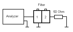
As an example, a two-section 165 MHz cavity filter was used. A scan from 150 to 180 MHz (500 points) was done by using a RigExpert antenna analyzer.
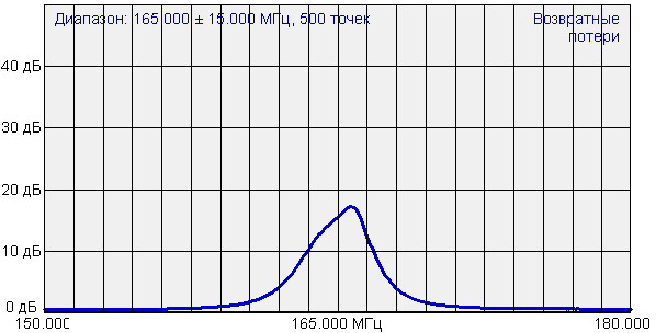
The AntScope shows the following RL (Reflection Loss) graph for this filter:
The data was saved to the 3-180-500.s1p file, then imprted into the myVNA software. The program outputs t(S11) and RL (Return Loss) at the same time. The TDR mode section of the help file describes how to do this.
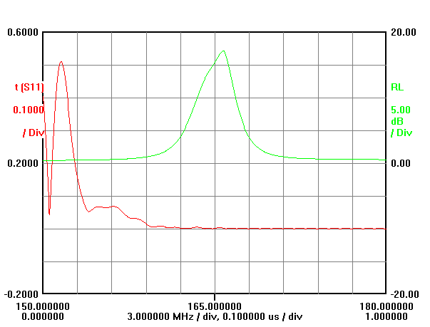
The red graph (horizontal axis is time, vertical axis is module of S11) has two dips: at 16 ns (resonance of the 1st section of the filter) and at 132 ns (2nd section).
And now the most interesting part. As described in the myVNA help file, by using a mouse the green graph may be shifted left or right, and the red graph will change accordingly. The first dip has minimum value when the center frequency is shifted to 165.75 MHz:

The second dip is mostly visible when the center frequency equals to 158.36 MHz:
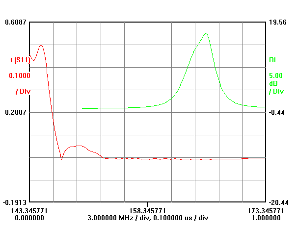
These are resonant frequencies of two sections of the measured filter. And now let’s do a routine work changing the center frequency from 155 to MHz with 1 MHz steps and saving results into the file (by using the Save TDR data to file option). The content of these file is then inserted into the MS Excel table.
Now we can plot a beautiful 3D graph. The X axis is time in microseconds, the Y axis is frequency in MHz, and the Z axis is module of S11 (which is plotted upside-down in logarithmic scale for better visibility).

The dips are now seen as peaks, which coordinates at Y axis correspond to tuning frequencies of two sections of the filter. Upper view:

This method of visualizing of characteristics of a filter allows identifying individual sections of a filter easily. Of course, instead of pasting data into the MS Excel file, a special software should be developed to perform all calculations automatically.
For sure, this method can also be used for testing and tuning duplex filters:
The analyzer should be connected to the antenna port of the duplexer. Load resistors should be used instead of the transmitter and the receiver. In this case, peaks will be located at the graph like shown at the following picture: bad or mistuned sections of the filter could easily be identified.
Denis Nechitailov, UU9JDR
17-Dec-2011